
Toshimasa Hashimoto
President, ai-Phase Co., Ltd.
Professor Emeritus, Tokyo Institute of Technology
Techniques for measuring thermal properties include weight- and length-based methods. Thermal analysis techniques such as differential scanning calorimetry (DSC) belong to the former category, and require a precision reference scale. On the other hand, in measurements of thermal conductivity, the sample thickness is the key question, and its mass is not required. Although these two types of measurement have traditionally been viewed as quite distinct, with separate textbook treatments and even separate academic societies, it goes without saying that actual thermal properties of materials reflect the qualities of both. Thermal energy exists primarily in the form of kinetic energy, such as the vibrational energy of crystal lattices or of electrons. However, both types of measurements must contend with the fact that energy cannot be measured directly. Specific heat capacity and thermal conductivity are physical properties related to thermal energy, and measurements of both quantities ultimately amount to observing the time variation of temperature after application of a thermal excitation. But what is temperature? It is a measurable intensive quantity defined in terms of fixed points and scales determined at international conferences; for example, in the past the Celsius scale was obtained by dividing the interval between the freezing and boiling points of water into 100 equally spaced subintervals. Again, the quantity that is substantively meaningful is the flow of heat, but heat flow is caused by a potential temperature gradient, not a thermal energy gradient (such as an enthalpy distribution). The conversion of heat to temperature is mediated by physical bodies—that is, matter—and the conversion coefficient is a physical property known as the specific heat capacity. As is true for measurements of mechanical or electrical properties, there are multiple ways to apply thermal excitations for measurement of thermal properties: via pulses (flash methods), via steps (hot wire methods), via oscillatory signals (temperature-wave methods), or via constant rates of temperature increase (DSC).
In previous work, we have proposed the use of temperature-wave thermal analysis as an effective method for measuring thermal diffusivity, particularly for thin samples with small volumes such as polymer thin films. In this method, a weak temperature wave with an amplitude of 1°C or less is applied to the sample, and the propagation of this wave is analyzed. The thermal conductivity λ can be obtained from the decay of the temperature-wave amplitude, while the thermal diffusivity α can be obtained from its phase shift. In 2002 we founded a university-based startup company (ai-Phase Co., Ltd.) to provide actual measurement instruments to the industrial world. Whereas commercial temperature-wave analyzers have the feel of testers, our instruments require no sampling and no experience to operate, and offer reduced energy consumption, higher convenience and a small footprint, enabling measurements right on the factory floor.
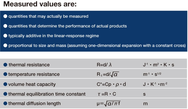
Quantities such as specific heat capacity and thermal conductivity, which are characteristic of the material in question and independent of its size or mass, are idealized values known as physical properties. On the other hand, in actual measurements and practical applications, we are interested in the properties of bodies of given sizes. For example, the goal of improving the insulation of a thermal insulator may be achieved either by choosing a material with lower thermal conductivity or by increasing the thickness of the material. The quantities that are meaningful in actual systems are functional values such as thermal resistance (the inverse of the thermal conductance). In Table 1 we have listed the units of some heat-related physical properties, with the corresponding functional values listed in Table 2. In an actual measurement, we determine the heat capacity or the thermal resistance, and then normalize using the mass or thickness of the sample to convert these functional values into physical properties. To make measurements requiring heat quantities, such as enthalpy of fusion or thermal diffusivity, we require standard substances whose properties are known in advance. Physical properties are important for theoretical reasoning and for comparisons between materials, but we must keep in mind that actual product designs are evaluated on the basis of functional values. In practical situations, cost limitations also come into play, and the material chosen is not necessarily that with the best physical properties. The fact that silver is not used for ordinary electrical wiring is a typical instance of this phenomenon.
Of all the thermal properties of materials, the distinction between thermal conductivity and thermal diffusivity is perhaps the most difficult to understand. Specific heat capacity and thermal diffusivity have unambiguous definitions as thermal properties; however, as noted above, the quantity of heat cannot be directly measured. In practice, the quantity of heat is converted to temperature using the specific heat per unit volume. The thermal conductivity is converted to thermal diffusivity and obtained by solving the temperature diffusion equation. If the thermal conductivity describes the speed at which heat travels, we might say that the thermal diffusivity describes the speed at which temperature travels.
This relation is summarized by the equation
λ=α•Cρ•ρ
The four physical properties in this equation are sometimes known as the four heat constants. When working with physical properties, we assume substances of uniform composition. Although hybrid materials such as multilayer systems may have functional values, strictly speaking we cannot assign physical properties to such systems.
Table 1
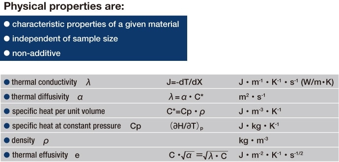
Table 2
A sinusoidal heat source applied to a given plane in a material (or to a given point in one-dimensional equations) produces waves that disperse in all directions; these are known as thermal waves. A good example of a thermal wave is the daily variation in the Earth’s temperature due to irradiation from the sun. Because the observable quantity that is actually measured is the variation in temperature, the term temperature waves is frequently used. In contrast to elastic or other types of waves, attenuation of these waves is extremely rapid. To quantify the distance over which a temperature disturbance propagates, we define the thermal diffusion length µ. For temperature waves with sinusoidal waveforms, the amplitude of a wave originating from a given point decays exponentially as the wave diffuses, and the thermal diffusion length is the distance at which the amplitude has decreased by the factor 1/e. The thermal diffusion length µ is defined as the square root of the quantity (α/πf ). For polymer materials, the diffusion length for temperature waves at 1 Hz is on the order of a few hundred microns. By varying the frequency, it is possible to vary the thermal diffusion length around a central value defined by the sample thickness d (i.e., around the point at which d/µ=1). At high frequencies, the thermal diffusion length is short; because the wave decays in the vicinity of the sample surface, we describe this condition by saying that the sample is thermally thick, and thermally thick conditions are well-suited to measurements of thermal diffusivity with little external disturbances. In the opposite limit of low frequencies, we speak of thermally thin conditions; in this case it is difficult to maintain a temperature difference between the front and back sides of a sample, but the system is easily influenced by environmental conditions—such as the presence of other nearby bodies—and it becomes possible to determine the thermal conductivity of materials in contact.
As shown in Figure 1, the instrument that we brought to market as ai-Phase Mobile 1 boasts a compact, lightweight design footprint, allowing the device to be used on-site at production facilities. The instrument consists of a sampleplacement unit and an amplifier unit; the sample unit may be inserted into a desiccator, glove box, or other similar chamber. The amplifier unit is equipped with oscillators for signal generation, AD converters, lock-in amplifiers, microcontrollers, temperature controllers, and other useful functions. This allows measurements of thermal diffusivity using only the device itself, with no external equipment required.
Figure 2 is a schematic cross-sectional image of the sample unit, comprising a micro-heater and a temperature sensor facing each other, with the sample mounted between them. A weak sinusoidal electrical power signal is supplied to the heater, producing a temperature wave over the sample surface. The sensor is a high-sensitivity resistive sensor which uses a preamp to amplify the weak signal before it is fed into a digital lock-in amplifier. The observed temperature signal is a mixture of the excitation temperature wave and background temperature signals such as the temperature of the room. In AC measurements, an advantage of lock-in amplification is the ability to extract and analyze the variation of just one specified frequency component of the signal, cancelling the contribution of room temperature variations—a major source of offse—as well as noise components, to achieve high sensitivity. By limiting the amplitude of the actually applied temperature wave to 1°C or below, we strongly suppress convection and radiation and ensure almost no damage to the sample. Moreover, the small sensor size of 0.25 × 0.5 mm allows the thermal diffusivity of extremely small sample regions to be identified.
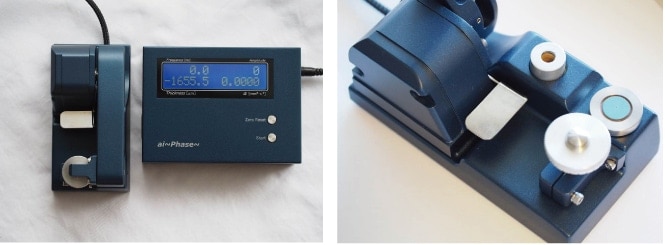
Fig 1. ai-Phase Mobile (Thin-film / thermal-diffusivity measurement model)
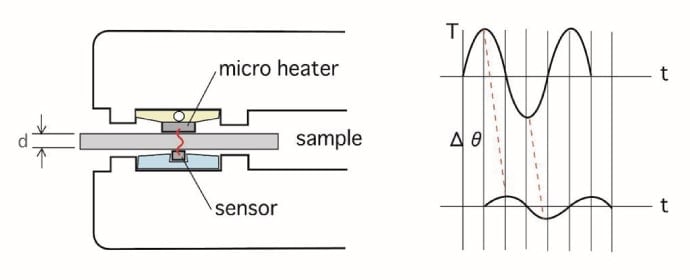
Fig 2. Schematic cross section of sample unit
By focusing on the phase shift between the front and back of the sample, in frequency regimes in which the ratio of the sample thickness to the thermal diffusion length is on the order of 3-4, we have—independent of the surrounding conditions—the following relation:
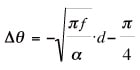
Here Δθ is the phase shift, α is the thermal diffusivity, f is the frequency, and d is the sample thickness. Thus, plotting the phase shift versus the square root of the frequency, and using separately measured values for the sample thickness, allows calculation of the thermal diffusivity. In this instrument, a differential transformer mounted on a moving arm is used to make successive measurements of the sample thickness, allowing monitoring of sample deformation even while measurements are in progress.
Figure 3 plots measured values of the phase shift versus the square root of frequency for pure copper samples of different thicknesses (approximately 2 mm and 0.1 mm). The solid line is a blank curve measured with no sample present; the influence of the environment (the heat capacity of the sensor and heater themselves, losses to lead wires, etc.) are visible particularly at lower frequencies. Subtracting the blank-curve contribution from the measured value yields a linear relationship between √f and Δθ, whose slope we determine in the appropriate frequency range. In this case we have two different thicknesses, and thus the appropriate frequencies differ; nonetheless, we obtain the same values for the thermal diffusivity. However, because the quantity of heat transport is not relevant in this case, we do not directly determine the thermal conductivity, and thus we use the formula above to convert values from thermal diffusivity. Because phase-shift measurements can be made for samples of varying thickness and thermal diffusivity, by varying the frequency between 0.02 and 2 kHz and matching the thermal diffusivity length with the sample thickness, it is possible to use the same instrument to measure thermal diffusivity for materials ranging from diamond to thermal insulators. This method may be applied to arbitrary materials with thicknesses ranging from the order of microns to around 3 mm (for thermal conductors) or around 1 mm (for thermal insulators). The quantity measured is the temperature resistance (the slope of the curves in the plot); for a substance of uniform composition, the sample thickness may be used to yield the material property of thermal diffusivity. The square of the slope is called the thermal equilibration time constant τ; this is the actual quantity measured by this instrument. The quantity τ has units of time; it represents the time required for signals to travel between the front and back surfaces of the sample.
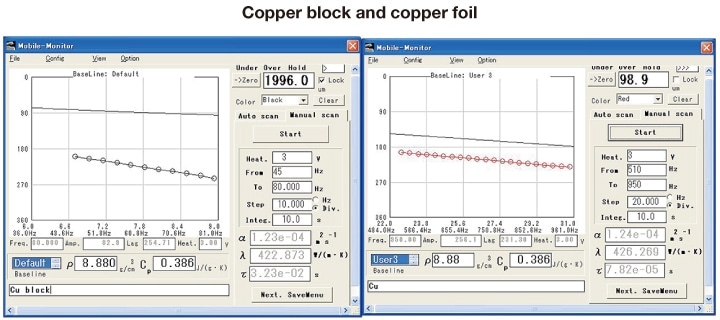
Fig 3. Plots of measured phase shift versus square root of frequency for pure copper samples
(thicknesses: approximately 2 and 0.1 mm)
In temperature-wave propagation analysis, the signal amplitude contains information on variations in the quantity of heat. In the regime opposite to that considered in the previous section—namely, low frequencies and thermally thin samples—the measurement system is strongly influenced by the thermal conductivity of external bodies. We now present a method that exploits the resulting amplitude decay.
Figure 4 is a schematic depiction of the heater/sensor configuration for the instrument we have developed. We use Peltier elements as heaters, with a high-heat-capacity aluminum block affixed to one surface as a heat sink. To the other surface we attach a temperature sensor, a reference sample (0.5 mm acrylic slab or similar), and a second temperature sensor, and pressure adhere these to the sample under measurement via a thin protective film (which also serves to improve the adhesiveness). In its entirety, the temperature-wave probe is stacked into an area of 30 mm2; the temperature sensor consists of a thermopile in which 5 thermocouples are arranged over a small 1×5 mm2 area near the center. The sensor surroundings function as a guard heater. The oscillator that supplies an AC signal to the heater, and the lock-in amplifier used to amplify the temperature output, are as described in the previous section.
As shown in Figure 5, the instrument consists of the amplifier unit and the sample-probe unit. Measurements are performed under conditions in which propagation of temperature waves on both surfaces of the reference sample are measured in the thermally thin regime. The sample to be measured is affixed to the back surface of the reference sample (seen from the heater side); assuming that a one-dimensional steady-state heat flow exists in the central portion of the sample, the amplitude of the temperature wave passing through the reference sample is sensitively influenced by the thermal conductivity of the measurement sample in contact with its back surface.
For measurements, the amplitude and frequency of the AC voltage signal supplied to the heater are fixed, and the rate of amplitude decay between the front and back sample surfaces is determined. The frequency is chosen to ensure that the amplitude decays by approximately 50% between the front and back sample surfaces. The temperature wave that passes through the reference sample and flows into the measurement sample falls to zero amplitude (in practice on the order of 0.1%) at some point inside the sample. We have confirmed that, for samples of a foam material of various thicknesses at a frequency of 0.05 Hz, there is no dependence on sample thickness for thicknesses above about 1 mm, and the amplitude decay rate becomes constant in this regime. This decay rate depends on the frequency of the temperature wave, the thermal resistance of the reference sample, and the thermal properties of the external bodies to which it is connected. In other words, the measurement amounts to monitoring a one-dimensional flow of heat by considering the temperature variation between the ends of a reference thermal resistor. From the amplitude decay rate we can determine the thermal impedance (a quantity which corresponds to the ratio of the heat capacity and thermal resistance, i.e., the thermal penetration coefficient); by comparing to amplitude decay ratio for substances of known thermal conductivity we can convert this value into the thermal conductivity.
Substances to which this method is applicable include foams—including inorganic materials—powders, compressed bodies, paper bundles, fabrics, polymer blocks, rubbers, liquids such as water and oils, and other substances with thermal conductivities in the range 0.02-5 W/(m•K). For powders or liquids, measurements can even be performed with the sample enclosed in a bag, as in Figure 5, and mutual comparisons can be conducted. Relative variations can be investigated using data associated with the interior of vacuum-insulating materials. Also, by varying the thermal resistance of the reference sample, the range of applicability of the method can be varied, with applications extending even as far as thermally conducting rubbers. Thus we have a revolutionary new measurement method that is simple to use and yields results in a matter of minutes.
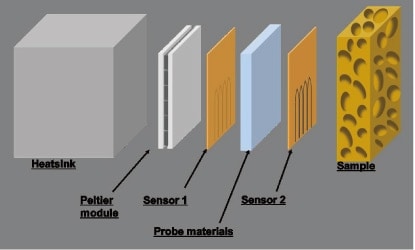
Fig 4. chematic depiction of heater/sensor configuration
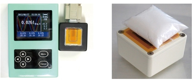
Fig 5. Full ai-Phase mobile instrument (bulk materials / thermal conductivity measurement model) and measurement of bagged powder sample
Thermal energy is energy that cannot be localized at any specific point, which makes measuring its velocity of motion (the thermal conductivity) extremely difficult. Many measurement methods have been proposed to surmount this difficulty, each involving tricks for regulating the thermal environment of the measurement sample. In temperature-wave methods, a weak sinusoidal excitation is applied and the amplitude decay and phase shift are measured. We showed that phase-observation techniques are stable methods that can be applied to arbitrary thinfilm samples. The simplicity and high speed of this approach make it easy to take tens or hundreds of measurements, allowing thermal diffusivity data to be treated statistically; the significance of this is that it allows thermal properties— which depend strongly on the state of the sample—to be treated as distributions. On the other hand, we also noted that methods based on amplitude decay use low-frequency excitations, making them applicable to thick samples of nonconductive materials and allowing direct measurement of the thermal conductivity. Thus we have demonstrated that, with the proper choice of frequency, temperature-wave methods may be used to measure the thermal properties of a wide range of samples.
Standardization is an unavoidable step in the process of achieving widespread adoption of any measurement technique, and to this end we submitted an ISO proposal for temperature-wave methods at the time when we launched our startup venture. After a long and arduous process, our proposal was accepted as a contribution from Japan, and in 2008 was officially recognized as ISO22007-3 (Phase-analysis method for thin films) in the field of thermal conduction in plastics (TC-61). An alternative amplitude-analysis version (ISO-22007-6) was also accepted. Although many methods exist for measuring heat conduction, the most efficient approach is to use standardized, systematic methods in a round-robin testing configuration, and in some cases comparisons between multiple measurement techniques are necessary. This means that expectation values inevitably get mixed with measured values; however, correct characterization of complex materials is also directly tied to safety considerations, presumably requiring the collection of large quantities of data. The problems posed by the science of heat are at once ancient and modern, and we believe that modern material engineering has entered an era in which he who masters heat masters materials. We hope the methods and instruments we have developed will prove to be valuable tools for developing new materials.
See more